Introduction to rpy2
This introduction is intended for new users, or users who never consulted the documentation but encountered blockers after guessing successfully their first steps through the API.
Getting started
It is assumed here that the rpy2 package has been properly installed. This will be the case if working out of one of the Docker containers available, of if the instructions were followed (see Installation).
rpy2 is like any other python package binding to a C library. Its top level can be imported, and the version obtained.
import rpy2
print(rpy2.__version__)
Note
The rpy2 version is rather important when reporting an issue with rpy2, or in your own code if trying to assess whether rpy2 is matching the expected version.
A utility module is included to report what rpy2’s environment.
python -m rpy2.situation
If unable to run python from the command line, or unsure about about to do it, the same information can be obtained from a Python terminal (or notebook).
import rpy2.situation
for row in rpy2.situation.iter_info():
    print(row)
rpy2 is providing 2 levels of interface with R:
- low-level (rpy2.rinterface, and rpy2:rinterface_lib)
- high-level (rpy2.robjects)
The high-level interface is trying to make the use of R as natural as possible for a Python user (something sometimes referred to as “pythonic”), and this introduction only covers that interface.
Importing the top-level sub-package is also initializing and starting R embedded in the current Python process:
import rpy2.robjects as robjects
R packages
R is arguably one of the best data analysis toolboxes because of the breadth and depth of its packages.
Importing packages
Importing R packages is often the first step when running R code, and
rpy2 is providing a function rpy2.robjects.packages.importr()
that makes that step very similar to importing Python packages.
from rpy2.robjects.packages import importr
# import R's "base" package
base = importr('base')

# import R's "utils" package
utils = importr('utils')
In essence, that step is importing the R package in the embedded R, and is exposing all R objects in that package as Python objects.
Note
There is a twist though. R object names can contain a “.” (dot) while in Python the dot means “attribute in a namespace”. Because of this, importr is trying to translate “.” into “_”. The details will not be necessary in most of the cases, but when they do the documentation for R packages should be consulted.
Installing packages
Knowing how to install R packages is an important skill to have, although not always a mandatory one if working out of an R installation designed to meet all reasonable needs for a task or a project.
Note
Package installation is presented early in the introduction, but this subsection can be skipped if difficulties such as an absence of internet connection, an uncooperative proxy (or proxy maintainer), or insufficient write priviledges to install the package are met.
Downloading and installing R packages is usually performed by fetching
R packages from a package repository and installing them locally.
Capabilities to do this are provided by R libraries, and when in Python
we can simply use them using rpy2. An interface to the R features is
provided in rpy2.robjects.packages (where the function importr()
introduced above is defined).
Getting ready to install packages from the first mirror known to R is done with:
# import rpy2's package module
import rpy2.robjects.packages as rpackages

# import R's utility package
utils = rpackages.importr('utils')

# select a mirror for R packages
utils.chooseCRANmirror(ind=1) # select the first mirror in the list
We are now ready to install packages using R’s own function install.package:
# R package names
packnames = ('ggplot2', 'hexbin')

# R vector of strings
from rpy2.robjects.vectors import StrVector

# Selectively install what needs to be install.
# We are fancy, just because we can.
names_to_install = [x for x in packnames if not rpackages.isinstalled(x)]
if len(names_to_install) > 0:
    utils.install_packages(StrVector(names_to_install))
The code above can be part of Python code you distribute if you are relying on CRAN packages not distributed with R by default.
More documentation about the handling of R packages in rpy2 can be found Section R packages.
The r instance
We mentioned earlier that rpy2 is running an embedded R. This is may be
a little abstract, so there is an object rpy2.robjects.r to make
it tangible.
This object can be used as rudimentary communication channel between Python and R, similar to the way one would interact with a subprocess yet more efficient, better integrated with Python, and easier to use.
Getting R objects
The __getitem__() method of rpy2.robjects.r,
gets the R object associated with a given symbol, just
as typing that symbol name in the R console would do it
(see the note below for details).
Example in R:
> pi
[1] 3.141593
With rpy2:
>>> pi = robjects.r['pi']
>>> pi[0]
3.14159265358979
Note
Under the hood, the variable pi is gotten by default from the R base package, unless an other variable with the name pi was created in R’s .globalEnv.
Whenever one wishes to be specific about where the symbol should be looked for (which should be most of the time), it possible to wrap R packages in Python namespace objects (see R packages).
For more details on environments, see Section Environments.
Also, note that pi is not a scalar but a vector of length 1
Evaluating R code
The object r is also callable, and the string passed in
a call is evaluated as R code.
The simplest such strings would be the name of an R object, and this provide an alternative to the method __getitem__ described earlier.
Example in R:
> pi
[1] 3.141593
With rpy2:
>>> pi = robjects.r('pi')
>>> pi[0]
3.14159265358979
Warning
The result is an R vector. The Section R vectors below will provide explanation for the following behavior:
>>> piplus2 = robjects.r('pi') + 2
>>> piplus2.r_repr()
c(3.14159265358979, 2)
>>> pi0plus2 = robjects.r('pi')[0] + 2
>>> print(pi0plus2)
5.1415926535897931
More complex strings are R expressions of arbitrary complexity, or even sequences of expressions (snippets of R code). Their evaluation is performed in what is known to R users as the Global Environment, that is the place one starts at when in the R console. Whenever the R code creates variables, those variables are “located” in that Global Environment by default.
For example, the string below returns the value 18.85.
robjects.r('''
        # create a function `f`
        f <- function(r, verbose=FALSE) {
            if (verbose) {
                cat("I am calling f().\n")
            }
            2 * pi * r
        }
        # call the function `f` with argument value 3
        f(3)
        ''')
That string is a snippet of R code (complete with comments) that first creates an R function, then binds it to the symbol f (in R), finally calls that function f. The results of the call (what the R function f is returns) is returned to Python.
Since that function f is now present in the R Global Environment, it can be accessed with the __getitem__ mechanism outlined above:
>>> r_f = robjects.globalenv['f']
>>> print(r_f.r_repr())
function (r, verbose = FALSE)
{
    if (verbose) {
        cat("I am calling f().\n")
    }
    2 * pi * r
}
Note
As shown earlier, an alternative way to get the function
is to get it from the R singleton
>>> r_f = robjects.r['f']
The function r_f is callable, and can be used like a regular Python function.
>>> res = r_f(3)
Jump to Section Calling R functions for more on calling functions.
Interpolating R objects into R code strings
Against the first impression one may get from the title
of this section, simple and handy features of rpy2 are
presented here.
An R object has a string representation that can be used directly into R code to be evaluated.
Simple example:
>>> letters = robjects.r['letters']
>>> rcode = 'paste(%s, collapse="-")' %(letters.r_repr())
>>> res = robjects.r(rcode)
>>> print(res)
"a-b-c-d-e-f-g-h-i-j-k-l-m-n-o-p-q-r-s-t-u-v-w-x-y-z"
R vectors
In R, data are mostly represented by vectors, even when looking like scalars.
When looking closely at the R object pi used previously, we can observe that this is in fact a vector of length 1.
>>> len(robjects.r['pi'])
1
As such, the python method add() will result in a concatenation
(function c() in R), as this is the case for regular python lists.
Accessing the one value in that vector has to be stated explicitly:
>>> robjects.r['pi'][0]
3.1415926535897931
There is much that can be achieved with vectors, having them to behave
more like Python lists or R vectors.
A comprehensive description of the behavior of vectors is found in
robjects.vector.
Creating rpy2 vectors
Creating R vectors can be achieved simply:
>>> res = robjects.StrVector(['abc', 'def'])
>>> print(res.r_repr())
c("abc", "def")
>>> res = robjects.IntVector([1, 2, 3])
>>> print(res.r_repr())
1:3
>>> res = robjects.FloatVector([1.1, 2.2, 3.3])
>>> print(res.r_repr())
c(1.1, 2.2, 3.3)
R matrixes and arrays are just vectors with a dim attribute.
The easiest way to create such objects is to do it through R functions:
>>> v = robjects.FloatVector([1.1, 2.2, 3.3, 4.4, 5.5, 6.6])
>>> m = robjects.r['matrix'](v, nrow = 2)
>>> print(m)
     [,1] [,2] [,3]
[1,]  1.1  3.3  5.5
[2,]  2.2  4.4  6.6
Calling R functions
Calling R functions is disappointingly similar to calling Python functions:
>>> rsum = robjects.r['sum']
>>> rsum(robjects.IntVector([1,2,3]))[0]
6L
Keywords are also working:
>>> rsort = robjects.r['sort']
>>> res = rsort(robjects.IntVector([1,2,3]), decreasing=True)
>>> print(res.r_repr())
c(3L, 2L, 1L)
Note
By default, calling R functions returns R objects.
More information on functions is in Section Functions.
Getting help
R has a builtin help system that, just like the pydoc strings are used frequently in python during interactive sessions, is used very frequently by R programmmers. This help system is accessible from an R function, therefore accessible from rpy2.
Help on a topic within a given package, or currently loaded packages
>>> from rpy2.robjects.packages import importr
>>> utils = importr("utils")
>>> help_doc = utils.help("help")
>>> help_doc[0]
'/where/R/is/installed/library/utils/help/help'
Converting the object returned to a string produces the full help text on the topic:
>>> str(help_doc)
[...long output...]
Warning
The help message so produced is not a string returned to the console
but is directly printed by R to the standard output. The call to
str() only returns an empty string, and the reason for this is
somewhat involved for an introductory documentation.
This behaviour is rooted in R itself and in rpy2 the
string representation of R objects is the string representation as
given by the R console,
which in that case takes a singular route.
For a Python friendly help to the R help system, consider the module
rpy2.robjects.help.
Locate topics among available packages
>>> help_where = utils.help_search("help")
As before with help, the result can be printed / converted to a string, giving a similar result to what is obtained from an R session.
Note
The data structure returned can otherwise be used to access the information returned in details.
>>> tuple(help_where)
(<StrVector - Python:0x1f9a968 / R:0x247f908>,
 <StrVector - Python:0x1f9a990 / R:0x25079d0>,
 <StrVector - Python:0x1f9a9b8 / R:0x247f928>,
 <Matrix - Python:0x1f9a850 / R:0x1ec0390>)
>>> tuple(help_where[3].colnames)
('topic', 'title', 'Package', 'LibPath')
However, this is beyond the scope of an introduction, and one should
master the content of the module robjects.vector before anything else.
Examples
This section demonstrates some of the features of rpy2.
Graphics and plots
import rpy2.robjects as robjects

r = robjects.r

x = robjects.IntVector(range(10))
y = r.rnorm(10)

r.X11()

r.layout(r.matrix(robjects.IntVector([1,2,3,2]), nrow=2, ncol=2))
r.plot(r.runif(10), y, xlab="runif", ylab="foo/bar", col="red")
Setting dynamically the number of arguments in a function call can be done the usual way in python.
There are several ways to plot data in R, some of which are presented in this documentation:
The general setup is repeated here:
import rpy2.robjects as robjects
from rpy2.robjects import Formula, Environment
from rpy2.robjects.vectors import IntVector, FloatVector
from rpy2.robjects.lib import grid
from rpy2.robjects.packages import importr, data
from rpy2.rinterface_lib.embedded import RRuntimeError
import warnings

# The R 'print' function
rprint = robjects.globalenv.find("print")
stats = importr('stats')
grdevices = importr('grDevices')
base = importr('base')
datasets = importr('datasets')
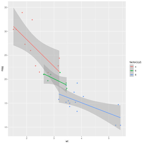
The setup specific to ggplot2 is:
import math, datetime
import rpy2.robjects.lib.ggplot2 as ggplot2
import rpy2.robjects as ro
from rpy2.robjects.packages import importr
base = importr('base')

mtcars = data(datasets).fetch('mtcars')['mtcars']
pp = (ggplot2.ggplot(mtcars) +
      ggplot2.aes_string(x='wt', y='mpg', col='factor(cyl)') +
      ggplot2.geom_point() +
      ggplot2.geom_smooth(ggplot2.aes_string(group = 'cyl'),
                          method = 'lm'))
pp.plot()
More about plots and graphics in R, as well as more advanced plots are presented in Section Graphics.
Warning
By default, the embedded R open an interactive plotting device, that is a window in which the plot is located. Processing interactive events on that devices, such as resizing or closing the window must be explicitly required (see Section Processing interactive events).
Linear models
The R code is:
ctl <- c(4.17,5.58,5.18,6.11,4.50,4.61,5.17,4.53,5.33,5.14)
trt <- c(4.81,4.17,4.41,3.59,5.87,3.83,6.03,4.89,4.32,4.69)
group <- gl(2, 10, 20, labels = c("Ctl","Trt"))
weight <- c(ctl, trt)

anova(lm.D9 <- lm(weight ~ group))

summary(lm.D90 <- lm(weight ~ group - 1))# omitting intercept
One way to achieve the same with rpy2.robjects is
from rpy2.robjects import FloatVector
from rpy2.robjects.packages import importr
stats = importr('stats')
base = importr('base')

ctl = FloatVector([4.17,5.58,5.18,6.11,4.50,4.61,5.17,4.53,5.33,5.14])
trt = FloatVector([4.81,4.17,4.41,3.59,5.87,3.83,6.03,4.89,4.32,4.69])
group = base.gl(2, 10, 20, labels = ['Ctl','Trt'])
weight = ctl + trt

robjects.globalenv['weight'] = weight
robjects.globalenv['group'] = group
lm_D9 = stats.lm('weight ~ group')
print(stats.anova(lm_D9))

# omitting the intercept
lm_D90 = stats.lm('weight ~ group - 1')
print(base.summary(lm_D90))
This way to perform a linear fit it matching precisely the way in R presented above, but there are other ways (see Section Formulae for storing the variables directly in the lookup environment of the formula).
Q: Now how to extract data from the resulting objects ?
A: Well, it all depends on the object. R is very much designed for interactive sessions, and users often inspect what a function is returning in order to know how to extract information.
When taking the results from the code above, one could go like:
>>> print(lm_D9.rclass)
[1] "lm"
Here the resulting object is a list structure, as either inspecting the data structure or reading the R man pages for lm would tell us. Checking its element names is then trivial:
>>> print(lm_D9.names)
 [1] "coefficients"  "residuals"     "effects"       "rank"
 [5] "fitted.values" "assign"        "qr"            "df.residual"
 [9] "contrasts"     "xlevels"       "call"          "terms"
[13] "model"
And so is extracting a particular element:
>>> print(lm_D9.rx2('coefficients'))
(Intercept)    groupTrt
      5.032      -0.371
or
>>> print(lm_D9.rx('coefficients'))
$coefficients
(Intercept)    groupTrt
      5.032      -0.371
More about extracting elements from vectors is available at Extracting items.
Principal component analysis
The R code is
m <- matrix(rnorm(100), ncol=5)
pca <- princomp(m)
plot(pca, main="Eigen values")
biplot(pca, main="biplot")
The rpy2.robjects code can be as close to the
R code as possible:
import rpy2.robjects as robjects

r = robjects.r

m = r.matrix(r.rnorm(100), ncol=5)
pca = r.princomp(m)
r.plot(pca, main="Eigen values")
r.biplot(pca, main="biplot")
However, the same example can be made a little tidier (with respect to being specific about R functions used)
from rpy2.robjects.packages import importr

base     = importr('base')
stats    = importr('stats')
graphics = importr('graphics')

m = base.matrix(stats.rnorm(100), ncol = 5)
pca = stats.princomp(m)
graphics.plot(pca, main = "Eigen values")
stats.biplot(pca, main = "biplot")
Creating an R vector or matrix, and filling its cells using Python code
from rpy2.robjects import NA_Real
from rpy2.rlike.container import TaggedList
from rpy2.robjects.packages import importr

base = importr('base')

# create a numerical matrix of size 100x10 filled with NAs
m = base.matrix(NA_Real, nrow=100, ncol=10)

# fill the matrix
for row_i in xrange(1, 100+1):
    for col_i in xrange(1, 10+1):
        m.rx[TaggedList((row_i, ), (col_i, ))] = row_i + col_i * 100
None
One more example
"""
short demo.

"""

from rpy2.robjects.packages import importr
graphics = importr('graphics')
grdevices = importr('grDevices')
base = importr('base')
stats = importr('stats')

import array

x = array.array('i', range(10))
y = stats.rnorm(10)

grdevices.X11()

graphics.par(mfrow = array.array('i', [2,2]))
graphics.plot(x, y, ylab = "foo/bar", col = "red")

kwargs = {'ylab':"foo/bar", 'type':"b", 'col':"blue", 'log':"x"}
graphics.plot(x, y, **kwargs)


m = base.matrix(stats.rnorm(100), ncol=5)
pca = stats.princomp(m)
graphics.plot(pca, main="Eigen values")
stats.biplot(pca, main="biplot")